Hi, this is Wayne again with a topic “The Excel HYPERLINK Function”.
In this article, I’m going to show you how to use the Excel hyperlink function, to create hyperlinks using a formula and I’m going to focus on three main uses of this interesting function. So here I am in a spreadsheet: it’s got a list of names and the companies they work for their company website, Etc, and I would like in column e to have actual working links to these websites. Let’S look at how to do that. I’Ll. Just click on Cell E2 type equals hyperlink, and now it’s required that I put in a link location, in other words, this information here, the URL or link location, and then I can optionally put in a comma and put in a friendly name for this website.

So, let’s do it here, I could just type in the link location if I really wanted to, but it’s easier just to click here on Cell D2. So that’s the link, location, comma and I do want a friendly name for this hyperlink and I can get the friendly name here: synth Point music, so I’ll just click on that or I could type in the cell reference C2. If I prefer at this point, I should put in my right parenthesis – I don’t really have to, but it’s good to get in the habit, I’ll tap enter on the keyboard and that quickly I’ve got a nice looking hyperlink, it’s got a friendly name, it doesn’t look Like a crazy long URL with https colon, all of that it looks nice and neat, but it is a hyperlink if I click on this it’ll. Take me to that URL now. At this point, I can use the autofill handle to fill this same formula notice, that the formula is here that I’ve typed into this cell E2.

If I double click on this little tiny green Square in the lower right corner, it’s very small. But if I double click on that, it will autofill this same formula all the way down the spreadsheet. If you don’t want to double click on the fill handle, if you prefer, you can click and hold the click and then drag down, and it does the same kind of thing.

I’M going to undo that, because double clicking is often a little bit faster. So I’ll. Just double click there, it autofills all the way down my spreadsheet and notice that each hyperlink perfectly matches both the link, location or URL and the friendly name. So at this point I could click here on, let’s say New Wave mountain and it opens up the website for this small business and I can visit that website. I’M going to close out of that to get back to my spreadsheet now. Some of you might be thinking.
Was it really worth setting up that formula and auto filling it down? Because all I really had to do to create a formula was copy paste in the URL or type it in and then after typing it in or pasting it in tap, enter on the keyboard notice that that automatically turns the link, location or URL into a working Link and it’s now clickable, I can click on it to open up this fantastic website that you should definitely only check out to learn about this awesome music. But I bet you can guess a couple of the advantages of using the hyperlink function. For one look: what happens if, let’s say cyberphonic music changes their website instead of cyberfon.net? Let’S say it becomes cybermusic.com. I can just tab over and look the URL in column e has automatically updated to the new URL. What if the company changes its name? I can change it here in column C tab over and it changes in column e. Another Advantage is that, because it uses the friendly name, you can make it look a little nicer, a little shorter and also sometimes you import data that someone else created or that came from the Internet or some other source, and it comes in not automatically being in Link format, and so this is a way for you to clean up your spreadsheet a little bit with a simple formula.
So that’s one way to use the hyperlink function in Excel. Let’S look at a second case in which you might want to use this function so here in column K. I have a list of email addresses.
What if I want to convert those into clickable email addresses, so that if I click on the email, it actually opens up my email program and opens up a message to this person to do this. It’S pretty similar to what I just showed, but I’m just going to click on Cell L2 type equals hyperlink and just like before Excel is expecting a link, location and a friendly name. Now, if I click on Cell K2, it’s not quite gon na work.
So I’m going to delete that instead, I’m going to put in quotation marks mail to colon, close quote and then I’ll put in the Ampersand or and symbol. And then at this point. Yes, I will click on Cell K2. So this is going to add the words mail to and colon to the beginning of this email address. Okay. Next, I want to put in a friendly name I’ll put in a comma Now.
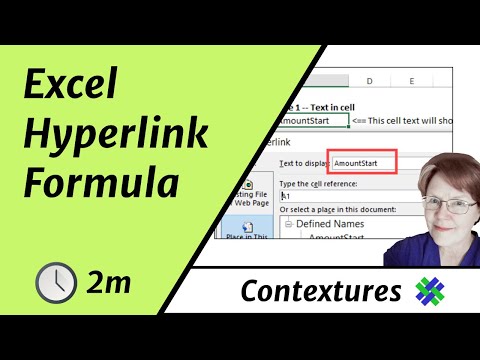
What do I do here? Should I just click on? Let’S say the person’s name I could, or maybe I’ll just type in the words send an email or better. Yet what if I were to type email, close quote and then I’ll use the Ampersand symbol again, but this time I’ll reference cell B2. So, let’s look at my formula up here in the formula bar, it says: equals hyperlink in quotes mail to colon, close quote and K2, which is the email address of Martin in this case comma, and then the friendly name is going to be email and the person’s First name so email, Martin, now there’s one little thing I forgot. I should have put a space after the word email. So I’ll put that in this formula looks great a little complicated, but it looks good I’ll tap, enter on the keyboard and look what I have using the hyperlink function. I’Ve pieced together a very handy link that not only opens up an email and an actual message to the specific person, but it also reminds me what the first name of that person is, which will help a lot. Okay, I’ll just double click on the autofill handle to extend this formula all the way down the spreadsheet. This is looking beautiful. Let’S move on to example, number three of how you can use the hyperlink function. As you can see, my spreadsheet is fairly long. It’S got 63 records and I would like to be able to quickly jump down to the second half of these records and I think I’ll put that link here in cell M1. So I click on it type in equals, hyperlink left parenthesis and I’m going to scoot over to the right a little bit.
So you can see this a little bit better and again, I’m going to put in quotation marks. But this time I would like to link to a specific cell in this spreadsheet, and so for that I need to put in a hashtag or a number symbol like this and then I’ll put in the cell reference. So a32, let’s say and then here I need to put the close quote comma and then I could put in a friendly name I don’t have to. But but what’s a friendly name I could put here.
Maybe something like quote jump to a32 close quote, and then I should put in my right parenthesis. Even though I don’t have to tap enter on the keyboard and I’ve got a nice link there, let’s see if it works, click on it and immediately it takes me to sell a 32, and I could have chosen any cell reference in this entire spreadsheet. Now some of you know that you can do a similar thing if you select a cell and go to insert link insert link, so that gives you similar capability, but in some cases you may want to Simply create that hyperlink using a formula. So those are three different ways that you can use the hyperlink function in Microsoft, Excel to create links that make the spreadsheet more useful and actually easier to use thanks for watching. I hope you found this tutorial to be helpful. If you did please like follow And subscribe, and when you do click the bell and you’ll be notified when I post another video, if you’d like to support my channel, consider clicking the thanks button below the video or you can support me through my patreon account or By buying Channel merch and you’ll see information about those options in the description below the video .