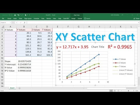
Hi, this is Wayne again with a topic “Create an XY Scatter Chart in Excel”.
In this article, i will show you how to create an xy scatter chart in microsoft excel and typically, when you create an xy scatter chart, the idea is you’re trying to investigate the relationship between two different values. So we have here in column b, the average weekly hours worked by a group of people and here in column c we have the average reported job satisfaction from 1 to 10 for the same group of people, and so i’d like to investigate how these values, the Average weekly hours affects these values, the average reported job satisfaction and in our xy chart. I would like these values to be our x values and these values to be our y values. Another way to think about the difference between these is that these values in column b – these are independent values or independent variables. In other words, they are the values that i think these values are affected by. These are independent.
These are dependent values, so i’m assuming that the average job satisfaction of the employees is dependent on the average weekly hours worked to help us explore this relationship between the two sets of values. Let’S create an xy scatter chart to do that. All i have to do is click anywhere inside the data, because this data is all together without gaps and also it helps that it’s all inside a table, but that’s not completely necessary, but because all the data is together. All i have to do is click anywhere inside the data and then go up here to the insert tab and look in the charts group. And here we have insert scatter, xy or bubble chart i’ll click. This arrow and i’m just going to select the most basic scatter chart, i click and that quickly i have an xy scatter chart for this data. Now it can be a little hard at first to understand what we’re looking at, i’m going to increase the size of this chart just by clicking and dragging the corner of the chart, and i could click here on the edge of the chart and drag it to A little bit better place.
I can also use this slider to decrease the zoom level in my spreadsheet, and then i can more easily click and drag and move this chart where i want it to go. So, as you can see, this xy scatter chart helps us to understand that the more hours worked by this group of employees generally speaking, the lower the job – satisfaction, at least at a certain point – and these are just random numbers that i put in. But you get the idea that it shows a trend now to help us understand that trend a little better.
We can add a trendline now that i have a chart in excel. If i have the chart selected, i can go up here to chart design and over here to the left, add chart element and i can select trendline by default. It has none, but i can change it to linear or any of these other listed kinds of trend lines i’m going to go with linear and it adds this nice dotted trendline to indicate the direction of the trend. Now, if i don’t like the way that trend line is set up, i can go back to the chart, design, tab and add chart element and i can go to trend line and then choose more trend line options. And here, if i’d like to, i can change the color of the trend line.
In my opinion, the blue dots kind of blend in with the rest of the blue on the chart, and it can be kind of hard to see that trend line. So i’m going to change the color, let’s say to purple, but you could change it to whatever you want. I could then also change the width of the trend line to make it easier to see. If i want to, i can change the dash type, which again may make it easier to read or may not.
It is possible to just also have a solid line if you prefer, if you want, you can also add and end arrow type, so that shows kind of the direction in which the trend line is headed. I’M going to take that off in my case, so now that we have a chart, we have a trend line. You don’t have to have a trend line if you don’t want to. Let’S look at some other ways that we could customize this chart to make it easier to read and understand, i’m going to select the chart again and then go up to chart design, add chart element and i want to add axis titles. Let’S start first with the primary horizontal axis title when i click on that it gives me this text box that i can click on, i can delete what’s there and i’ll, replace it with hours worked and then i could do the same thing again. Chart design add, chart element axis titles and this time primary vertical and i’ll triple click on that, and it highlights all of the text in that vertical axis title and then i can type job satisfaction. Another thing i can do to make this chart more readable easier to understand is: i could eliminate unnecessary parts of the chart so, for example, because no one in this group is working 30 hours or fewer, i’m going to go in and make the minimum number 30. I’Ll tap enter and the chart adjusts, i think, that’s improved the chart.

The data now fills more of the center of the chart. I think it looks good if i wanted to. I could do the same thing with the vertical numbers: just left, click on them and then right click format axis and i could change the minimum value. But i’m happy with the way it is notice whenever you create a chart in excel that we do have some other options here at the right.
Instead of going up here to chart design and clicking add chart element, i could have clicked here on this plus sign to add data labels, chart titles trendlines a legend and more so definitely check out this plus sign. That appears in the upper right corner of your charts in excel. That’S where you can easily and quickly add chart elements. We also have this paintbrush icon.

If you click on that, it gives you some chart. Styles, that you can choose from this doesn’t change the data itself, but it can change how the data looks in your spreadsheet. We also have some color options, so you could change the color scheme of your chart, so this button here just helps us to make our chart look more visually, appealing and sometimes easier to read, underneath that we have chart filters – and this can help us – as it Says here, edit the data points and names that are visible on the chart. So that’s another thing that you can adjust and work with in your excel chart, going back to the chart, design, tab, you’ll notice that you still have those same chart styles that we found here, but we have them on the chart, design tab. We also have some other options here that are worth looking at, including changing the chart type.
Let’S say this xy scatter chart doesn’t quite do what you think it would. You might want to switch to a different kind of scatter chart or a completely different chart altogether and then finally, we do have a move chart button. This makes it really easy to move your chart to a new sheet if you’d, like so i’ll, move it to a sheet called chart one. I click. Ok and now i have a new tab down here in the lower left corner. Here’S my spreadsheet, that has the data for the chart and then the chart itself is on a different tab. So that’s how you would create a simple xy scatter chart in microsoft, excel to help investigate the relationship or the correlation between two different sets of values.
Thanks for watching, i hope you found this tutorial to be helpful. If you did please like follow and subscribe, and when you do click the bell so you’ll be notified. When i post another video, if you’d like to support my channel, consider clicking the thanks button below the video or you could support me through my patreon account, or by buying channel merch and you’ll, see more information about those options.
In the description below the video .