Hi, this is Wayne again with a topic “Rank Your Excel Data with the RANK Function”.
In this Excel video, I will show you how to use the Excel rank function to quickly rank a series of numbers. So here we have a spreadsheet with a list of students and their test scores on a recent test, and you can see that here I’ve used the max function and the Min function to identify the highest score and the lowest score. But what about the second highest? Third, highest, Etc: let’s figure that out and we’re going to use one of two functions in Excel: either rank or rank dot EQ. So, as you can see, the test score data in the spreadsheet happens to be in a table. This area here is a table.
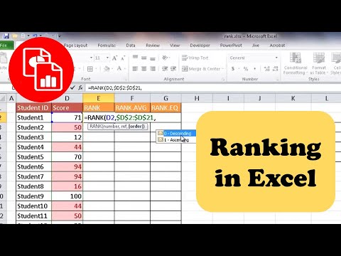
That’S okay, but I’ll click here on H2 and I’ll type in equals Rank, and you can see that there are three different rank functions that appear we’re going to want to use either rank or rank.eq. In this case, I’ll just use rank left parenthesis now Excel is expecting a number, and in this case it’s the test score number. So I’m going to click here on G 2 and then I’ll put in a comma next Excel wants to know. Okay. So this number, what is its ranking as compared to what other numbers? So I’m just going to select all of column G by clicking on the letter G and then I could end the formula there with the right parenthesis. I’Ll go ahead and tap enter on the keyboard and you can see what happened it calculated the ranking and not just for Albert.

It actually calculated all the way down the table now. The reason it did. That is because my data was in a table. Let’S try. The same thing again, but this time with a simple range: this is a range of data.

Let’S try it again I’ll just click on H2 equals rank left parenthesis, it’s looking for a number, it’s this number comma and I’m comparing this number to what range of numbers. Well, all of column G, so I click on G to select the entire column. Now you may notice it looks a little different here.
The formula does, and the reason for that is because I’m working in a Range this time a range of data, not an official table. Now I mentioned that. That’S all you have to do at this point I could put in the right parenthesis: tap enter and be done, but there is actually one more step that you may want to take. If you put another comma in the formula, you’ll notice that there’s an option for how to rank the data, do you want to descend? In other words, the highest test score would be number one and it would go down from there to the lowest number to the lowest test score. Or do you want to ascend? Do you want the highest test score to have the higher number in the rank? I’M going to put in descending right parenthesis, tap enter and I get the same result you can see back here in my table Albert got a rank of nine and in the range he also got a rank of nine now, because I’m not working in a table In order to apply this same formula all the way down the spreadsheet, I just need to double click on the autofill handle. As long as I have H2 selected I’ll, just double click on that and the formula is apply slide all the way down the spreadsheet.
So now I’m going to click on H2 and I’m going to go up here to the formula bar. This is a great bar here in Excel. It makes it easier to edit your documents and I’ll just switch that 0 to a 1 tap enter, and now the ranking will be ascending. Now I need to be sure and double click on the autofill handle again to update the numbers.
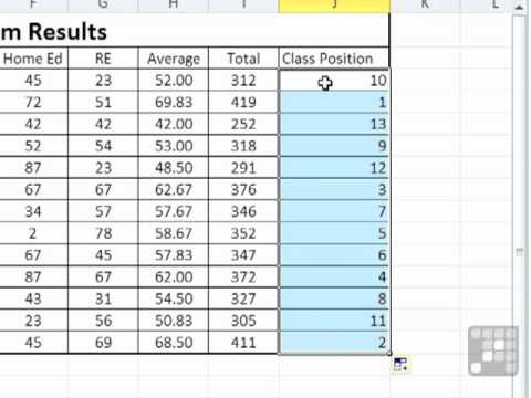
Otherwise, the only rank that would have changed would have been H2. So now you can see that the worst score is listed as rank number one, and so that’s the difference between ascending and descending. I just hit undo a couple of times to go back to descending order. Now I’m going to switch back here to the spreadsheet that has a table just to point out that, yes, the highest score is ranked number one.
The second highest score of 99 has the second Rank and third and so on. So this worked great but notice that some of the students got the exact same score. Griselda and Albert both got 84.. So how does Excel handle that with the rank function? If you look closely they’re both ranked as the ninth highest score, but as you look in the rest of the table, you won’t find a tenth ranked score.
There is no 10, it just skips 10 and it actually skips 11 as well. Why? Because there’s a third person who also got 84 and then it resumes with 12, 13 and so on. So that’s important to recognize that if you have ties in your rankings there will be certain numbers that will be skipped now, there’s one more important thing for you to understand.
If you remember, I talked about how there are two different Excel rank functions that you can use in this case, the one that we used just a minute ago was rank so equals rank, but if you’ll notice there is a little warning next to the rank function. Sometime in the future, Excel is likely to remove the rank function from Excel, so you may want to get used to using instead of rank, rank dot, EQ so I’ll, just type in rank.eq left parenthesis. What’S my number it’s this number here, comma? What am I comparing that number to all of the other numbers in column, G, comma? Do I want the rankings to be descending or ascending, and of course I could have just not put the comma in. I could have just hit enter, but I’ll go with the default, which is 0 descending right. Parenthesis tap, enter on the keyboard and so the results of the formula using the rank, dot, EQ function. The results are identical to when I used simply the rank function. So the results are the same, but it is important that you know that, eventually, that rank function will disappear out of excel thanks for watching. I hope you found this tutorial to be helpful. If you did please like follow And subscribe, and when you do click the bell and you’ll be notified when I post another video, if you’d like to support my channel, consider clicking the thanks button below the video or you can support me through my patreon account or By buying Channel merch and you’ll see information about those options in the description below the video speaking of patreon, I want to give a quick shout out to my five dollar patreon supporters.
Thank you. So much for all you do to support the channel. .